$\newcommand{\deriv}[2] {\frac{\partial #1}{\partial #2}}$

Lagrangian Mechanics

Classical approach

Is another formulation of Classical Mechanics.

This approach is very different from that of Newtonian mechanics, although it gives rise to an equivalent theory and solves the same problems. Firstly, the problems are rewritten in terms of generalized coordinates, not necessarily spatial (they can be distances, angles, etc.) and not necessarily Cartesian (polar, cylindrical or any other coordinate system that is convenient for solving the problem).

Such coordinates give rise to an abstract manifold denoted normally by $M$ or $\mathcal{C}$ (configuration space) specific to each problem, in which each point represents a state of the system under study (a combination of particle positions, positions and angles of rigid solids, velocities, etc.). A curve $\alpha: I\subseteq \mathbb{R} \to M$ represents a possible evolution of the system, and the generic problem of mechanics is to find which curve represents the actual evolution for a point $(p_0,v_0)\in TM$ of the tangent space, with $\alpha(0)=p_0$ and $\alpha'(0)=v_0$.

The principle of Lagrange and Hamilton, or the principle of least action, states that such a curve will be the one that minimizes the amount of "total Lagrangian". That is, for the system in question, a function

$$ L: TM \to \mathbb{R} $$

is defined that measures, for each $(p,v) \in TM$, the "toll to pay" for passing through a point $p$ with velocity $v$.

Any curve-evolution $\alpha$ has an "accumulation of Lagrangian" given by

$$ J(\alpha)=\int_I L(\alpha(t), \alpha'(t)) dt $$

We assume that the solution curve is the one with the lowest or highest $J(\alpha)$ (this is the principle of least action). We also assume the form of the function $L$. These assumptions arise, like everything in physics, from the observation of nature.

Personal idea: I visualize the Lagrangian as a toll that must be paid for taking a certain path at a certain speed. We must try to minimize the payment (or sometimes maximize it). From this point of view, the Lagrangian is like a kind of Riemannian metric, and we are computing a geodesic. This is not, of course, the case except in some cases. I think this has to do with Finsler manifolds...

Therefore, every system of Lagrangian Mechanics is a particular case of a variational problem.

A way to find the minimum or maximum of $J$ is resolve the Euler-Lagrange equations:

$$ \frac{d}{dt}\left( \deriv{L}{\dot{q}^k} \right)=\deriv{L}{q^k} $$

This equation implies Newton second law when we take $L=\dfrac{1}{2} m \dot{x}^2-V(x)$, where $V$ is the potential of the force:

$$ \deriv{L}{\dot{x}}=m\dot{x} $$ $$ \deriv{L}{x}=-\deriv{V}{x}=F $$

$$ m\ddot{x}=F $$

Jet space approach

From the point of view of the jet bundles, we have what follows.

We have the configuration manifold $M$ and the infinite jet bundle $J^{\infty} (\mathbb{R},M)$. We have also the total derivative operator $D_t$.

Physics is introduced by the Lagrangian, which is an horizontal 1-form on the first order jet bundle $J^1(\mathbb{R},\mathbb{R})$ (maybe related, variational bicomplex):

$$ \lambda=L(t,u,u_1)dt. $$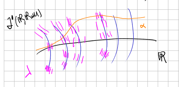

Given a general curve $\alpha:I \to J^1$ we can compute $\int_{\alpha} \lambda$.

The important sections $\phi$ of $\pi:\mathbb{R}\times M\to \mathbb{R}$ (i.e., curves of $M$) are those which extremizes the functional

$$ S[\phi]=\int_T (j^1\phi)^*(\lambda) $$

being $T$ a closed interval of $\mathbb{R}$ and $j^1\phi$ the prolongation to the first order jet space (holonomic section). Therefore we have a variational problem.

The condition of $\phi$ extremizing this functional is equivalent to satisfying Euler-Lagrange equation, a second order ODE.

So we can define a map

$$ \Delta: J^2 (\mathbb{R},M) \longmapsto \mathbb{R} $$

that codifies the Euler-Lagrange equations associated to a Lagrangian $\lambda.$ (I think the actual object is not a "map" but a 2-form called the Poincare-Cartan form $\Omega_{\lambda}$.)

Therefore, our Lagrangian (and the principle of least action) defines a submanifold $S_{\Delta} \subset J^2(\mathbb{R},M)$ given by

$$ \Delta(t,u,u_1,u_2)=0. $$

Given a curve $\alpha: \mathbb{R} \mapsto M$, its prolongation

$$ pr(\alpha): \mathbb{R} \longmapsto J^2 (\mathbb{R},M) $$

may or may not live inside $S_{\Delta}$. Of course, $\alpha$ is a critical curve when it does.

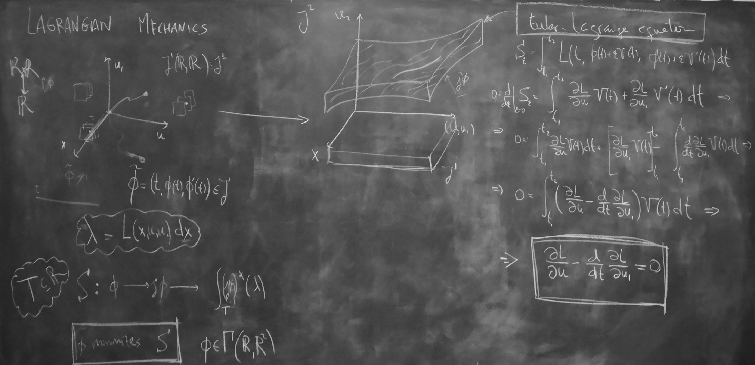
(pizarra_016)

I have a visualization of the relation of minimizing the action with satisfying Euler-Lagrange in xournal_154, although it is done from a "discrete point of view".

On the other hand, I guess that a group symmetry for the Lagrangian $L: J^1 (\mathbb{R},M)\mapsto \mathbb{R}$ implies that this group leaves invariant the submanifold $S_{\Delta}$, but I have to proof it. I have to learn more on variational symmetrys.

Other facts

Besides the equations of motion you have holonomic constraints or nonholonomic constraints.

Several Lagrangians can give rise to the same theory: equivalent Lagrangians

Worked example

________________________________________

Author of the notes: Antonio J. Pan-Collantes

antonio.pan@uca.es

INDEX: